Motivation

News is very important. A lot of important decisions are made based on the latest news. With the technology today, we are able to access all kinds of news resource or social media, such as Twitter, SFGate, New York Times, very easily. But the problem is it becomes very unlikely that a person can read all the news everyday in a limited amount of time. And this is why we need machine learning to help us to do the work.

In this project, I am trying to use topic modeling to capture the evolution of news topics in San Francisco from 2013 to 2015.

Topic modeling

Topic modeling is one of the important subjects of natural language processing. The goal of topic modeling is to capture the topics from a set of documents and cluster the documents by their topics. The basic methods for topic modeling include: LSI (Latent semantic indexing ), NMF (Non-negative matrix factorization), LDA (Latent Dirichlet allocation) and so on. Due to the fact that LDA doesn’t have to deal with large matrix processing (SVD), it has the fastest process speed and has the most protential to achieve dynametic (real-time) topic modeling. It is also the method that will be used in this project.

Basic idea of LDA

The theoretical detail of LDA will not be discussed in this blog. But the basic idea of LDA is that, it assumes a document is characterized by a particular set of topics and a topic is characterized by a distribution of words. Both the topics in a document and words in a topics follow the Dirichlet distribution. For any word in a document, it comes from a Multinomial trail of topics and words. By doing LDA analysis, we will be able to get a probability distribution of topics in each document and also a probability distribution of words in each topic.

Data source

The data of this project came from the New York Times API. With time range 2013 to 2015 and search query of San Francisco, about 10300 news articles were obtained. Please check the ipython notebook for the code of getting the data https://github.com/RuiChang123/Natural_language_processing_project/blob/master/NLP_project.ipynb

Preprocessing

Preprocessing is a very important part of topic modeling. In this project, preprocessing includes tokenizing, filtering numbers and date, filtering stop words and stemming. I also started with filtering words in more than 75% or less than 10 of the documents. During the process of training the model, stop words were updated and different word-filtering parameters were tested. The code for token processing is also in the ipython notebook

Topic modeling

After preprocessing, it is time to do the topic modeling. Python package gensim is used to achieve this process. For each document, we will get the probabilities of each topics within this document. Because topic modeling is an unsupervised learning process, the most difficult part is to decide the number of topics.

Choosing the number of topics

Actually, in my opinion, there is no correct answer of how many topics there are. Several small topics can be grouped into a bigger topic and a big topic can be seperated into several small topics. For example, the topic of sports can be seperated into football and baseball (like zoom in, zoom out). How do we choose the number of objects totally dependents on the purpose of the project. In this project, I tried to choose the number of topics so that each topic represents a quite different as each other. In python, there is a package called gensimvis https://github.com/bmabey/pyLDAvis which helps us to evaluate the topics very easily. This packges allows us to visualize the topics in a 2D plane. The distance between the topics is calculated based on the Jensen-Shannon divergence distance metric. As mentioned above, the assumption of LDA is that one topic is a distribution of terms. Jensen-Shannon divergence (JSD) is a metric that can be used to calculate the distance of two distributions. https://en.wikipedia.org/wiki/Jensen–Shannon_divergence This package also has a nice interactive chart that shows the top 30 terms in each topic.

With the help of gensimvis and after trying different number of topics with different word-filtering parameters, I finally chose the number of topics to be 10. The 2D plot of the topics with gensimvis were shown below.

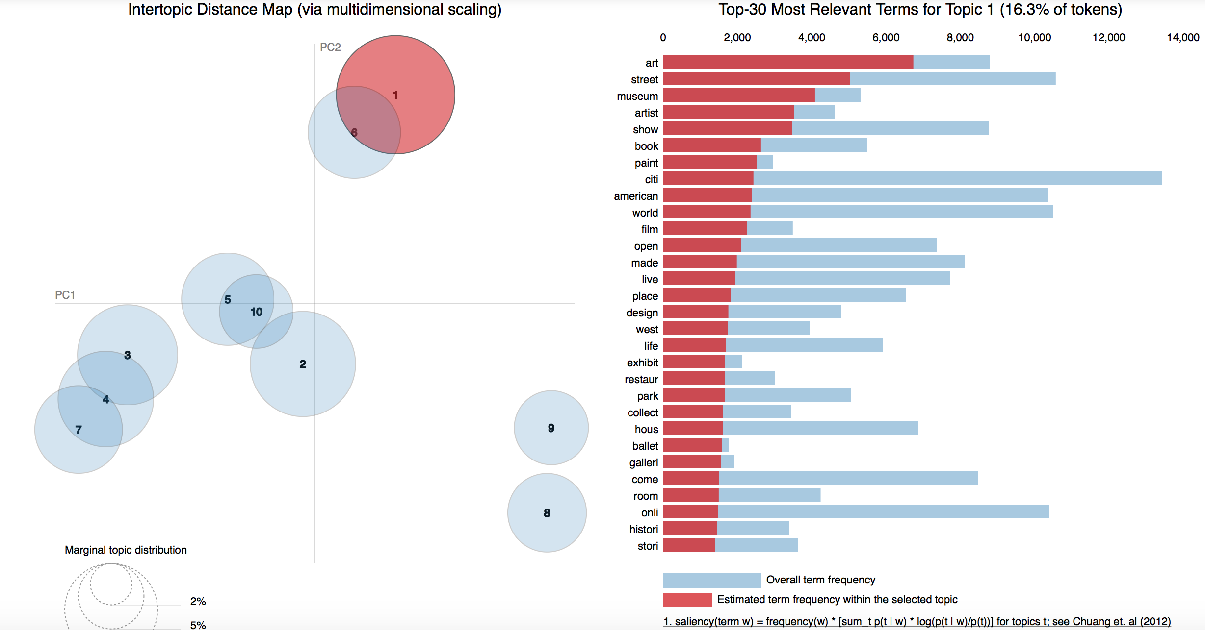
The topics were: Art; Music; Medical; Technology; Football; Government; Baseball; Family; Finance; Crime

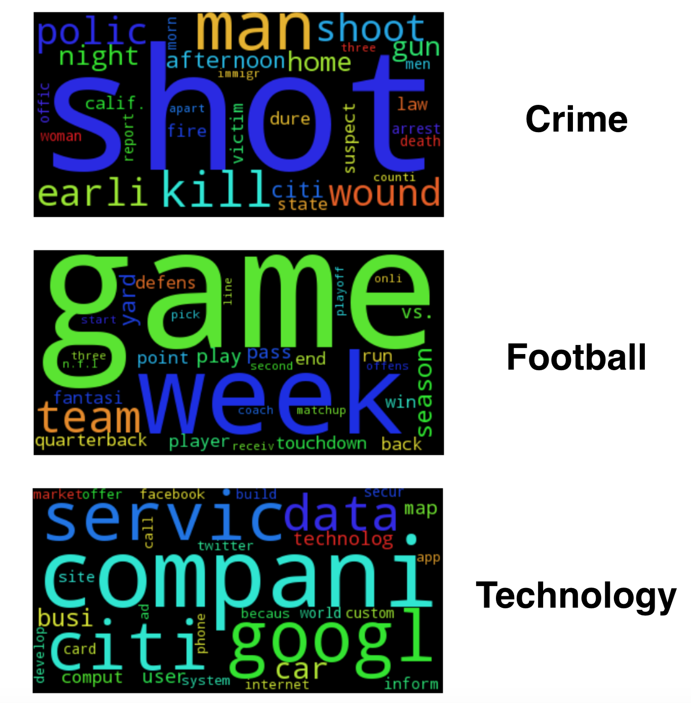
Word cloud

Word cloud is a nice way to look at the words in topics. In word cloud, a word with higher probability has bigger size. The plot below shows the words of 3 topics with the top 30 words using word cloud.

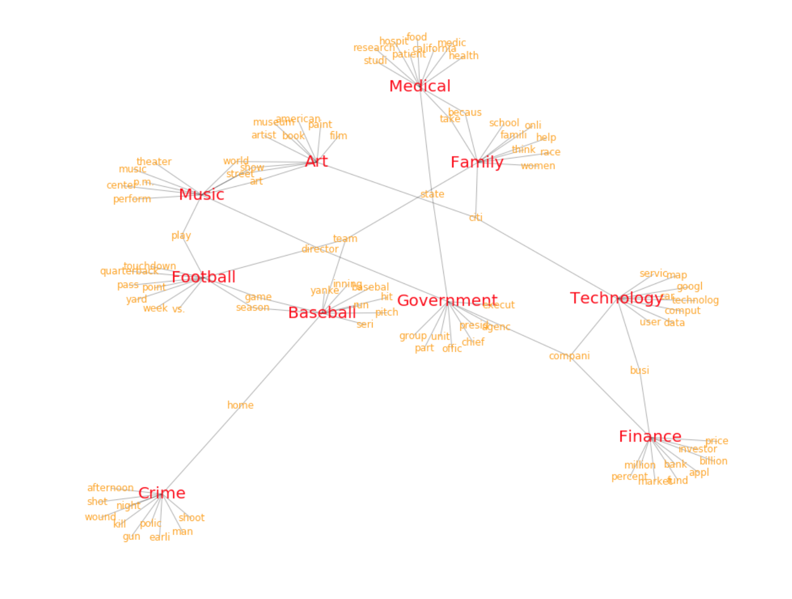
Topic-word network

We can also visualize the network of topics and words. From the network we can see how different topics connect with each other with common words. The network below shows the topics with top 10 words.

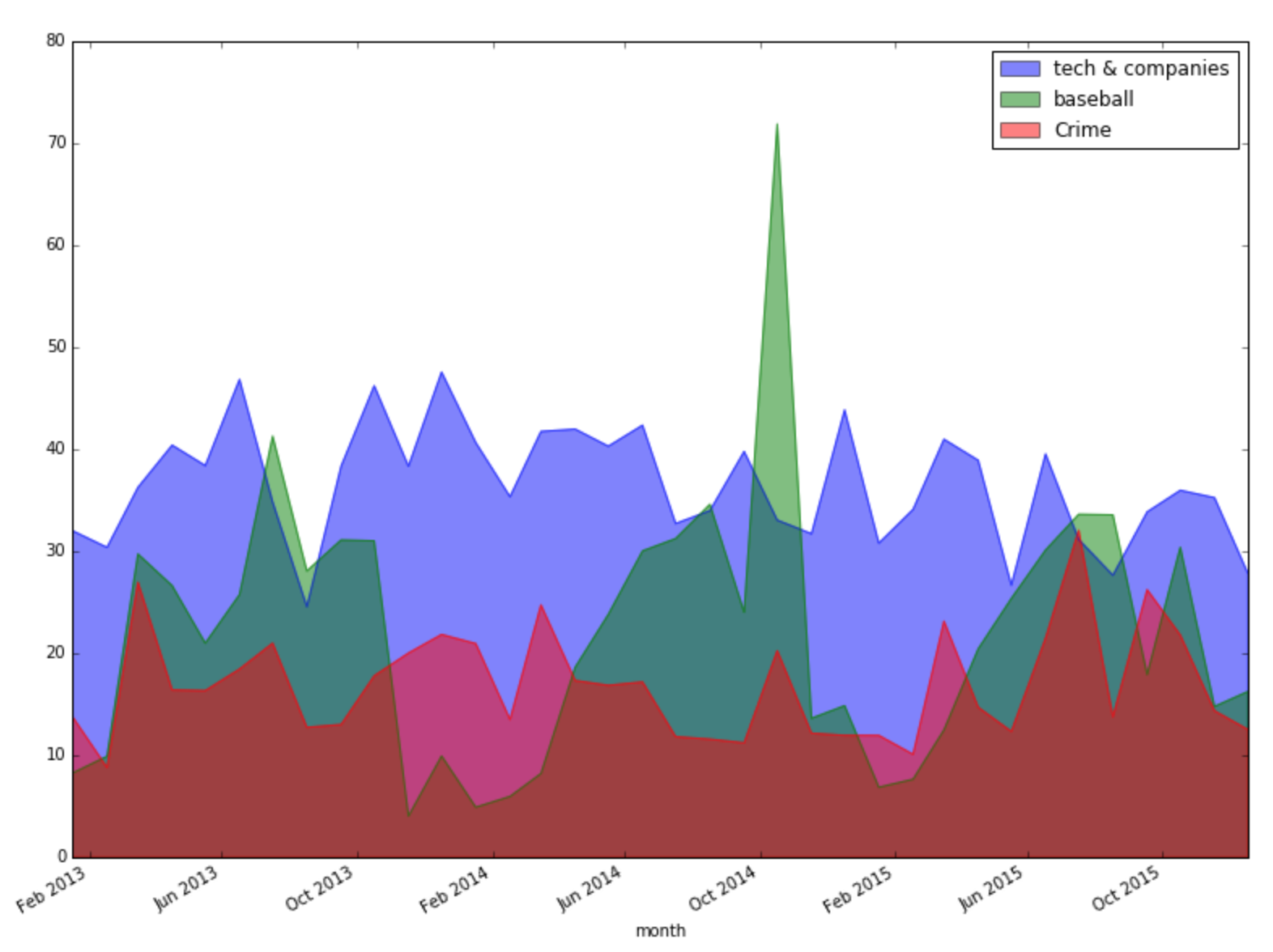
Topic evolution

After deciding the topics, it is time to study the evolution of topics vs. time. Keeping in mind that each document has more than one topics, I didn’t assign the articles to one topic that has the highest probability. Instead, I considered the contribution of this article to all the topics by getting the probabilities of all the topics in this article. The plot below shows the evolution of three topics. The topics about baseball show very clear seasonal change. The topic about technology kept a very high level because San Francisco has a lot of tech companies.

Conclusion

Topic modeling by computer itself is not an easy task. In this project, there was still a lot of manual work involved, especially choosing the number of topics. If the topics doesn’t change, it is ok to train the documents once, find the right number of topics and when a new document comes, just find the topic distribution using the trained model. But if we need to abandan old topics and find new topics as the time goes, we must find a good way that allows computers to decide the number of topics automatically.